The Legendre Transform: Intuition, Examples, and the Thermodynamic Connection

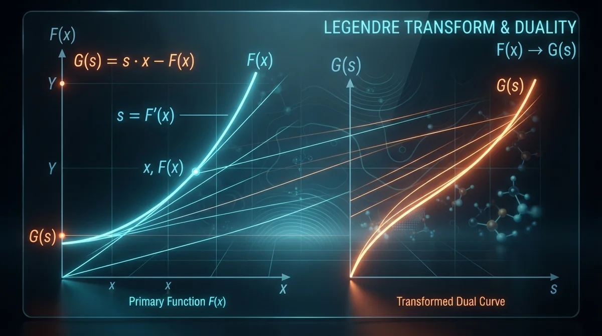
The Legendre transform is a standard tool for "reexpressing the information carried by a function from the perspective of another control variable, or covariable." This article explains step by step why the tool is needed, how it works through intuition and equations, and why it matters in physics, especially statistical thermodynamics. Each step uses concrete examples and analogies where possible to build an intuitive grasp of the core concept.

A common first question about the Legendre transform is simple: "What do we gain by introducing a different variable instead of the original one, and is the original information lost?" Answering it requires examining two points. First, is the original function sufficiently convex for a one-to-one correspondence between its derivative and its original variable? Second, which variable is easier to handle experimentally or theoretically? The following sections treat these questions more rigorously and use the geometric intuition of a tangent and its intercept to show why the formula arises naturally.

1. Problem setup and geometric intuition

Problem: Suppose quantity $F$ depends on independent variable $x$, so $F=F(x)$. In practice, however, its slope $s=dF/dx$ may be easier to measure or control than $x$ itself. We then want a new representation $G(s)$ whose independent variable is $s$. The key requirement is that mapping $x\mapsto s$ have an inverse. Mathematically, a convexity condition such as

$\frac{d^2 F}{dx^2} > 0$

makes $s$ and $x$ correspond one to one.

Geometric intuition: Draw a tangent at a point on the original function $F(x)$. The tangent's slope is $s$. Define the point where the tangent meets the $y$ axis, at $x=0$, as $-G$. The tangent equation gives

$\frac{F - (-G)}{x} = s$

and therefore

$G = s x - F.$

The important point is that once $x$ has become a function of $s$, the precise definition of $G$ is

$G(s) = s\, x(s) - F\bigl(x(s)\bigr).$

This is not a simple substitution but "repackaging the same information." Under sufficient convexity, applying the Legendre transform again recovers the original function.

Term explainer: Legendre transform

Simple definition: A mathematical procedure that transforms a function $F(x)$ into a new function $G(s)$ whose independent variable is its derivative $s=dF/dx$. Everyday example: It resembles describing terrain in terms of its slope on a contour map rather than the original elevation. The description is reorganized around the location of each particular slope instead of the terrain's height.

Why is this reexpression useful? Consider a situation in engineering or experimentation where it is easy to control or measure the force applied to a system, but difficult to handle the corresponding position directly. A representation using force as the independent variable—such as the Legendre transform of a potential for an elastic system—is then more natural. This perspective connects directly to the practical reason for moving between "energy representations" and "free-energy representations" in thermodynamics.

2. Harmonic potential example—what information the transform preserves or loses

As a concrete example, consider the harmonic potential

$U(x) = \tfrac{1}{2}k\bigl(x - x_{\min}\bigr)^2.$

If an external force $f$ is applied, equilibrium requires the sum of the internal force derived from the potential and the external force to be zero. The force from the potential is $-dU/dx$, so static equilibrium is

$-\frac{dU}{dx} + f = 0\quad\Rightarrow\quad \frac{dU}{dx} = f.$

Solving gives

$x(f) = \frac{f}{k} + x_{\min}.$

Now call the Legendre transform of $U(x)$ by the name $V(f)$. By definition,

$V(f) = f\, x(f) - U\bigl(x(f)\bigr).$

Direct calculation, after simple algebraic rearrangement, gives

$V(f) = \frac{1}{2}\frac{f^2}{k} + f x_{\min}.$

After the transform, we can also verify that

$x(f) = \frac{dV}{df}.$

Two observations are important in this example.

• The Legendre transform preserves information by reexpressing the position-slope pair $(x, s)$ as a slope-position pair $(s, x)$. Applying the transform twice recovers the original function.
• If the original $U$ is instead written only as $U[x(f)]$ in terms of $f$, information in a constant term—here $x_{\min}$—may be lost. A simple substitution and a formal Legendre transform therefore differ in information preservation.

The example clearly demonstrates both "why a precisely defined transform is necessary" and "which information is preserved or removed in the transformation." This distinction should be considered when deciding which variable to use as a controllable parameter in practice.

3. The connection to the Laplace transform and statistical thermodynamics—a shift toward the partition function

Although it is not mathematically identical to the Legendre transform, the Laplace transform plays a conceptually similar role in statistical thermodynamics. Given the microstate density $W(U)$, the phase-space volume of states whose internal energy is near $U$, the partition function is defined by

$Z(\beta) = \int W(U)\, e^{-\beta U} \, dU,$

where $\beta = (k_B T)^{-1}$. The partition function is a function whose independent variable is temperature, or $\beta$, and describes a system from the "temperature rather than energy" perspective.

Using the Bromwich integral, the inverse Laplace transform rewrites $W(U)$ as

$W(U) = \frac{1}{2\pi i} \int_C Z(\beta)\, e^{\beta U} \, d\beta,$

where path $C$ is a suitably selected line in the complex plane. The partition function also connects to Helmholtz free energy $F$. Defining $\mathcal{F} \equiv \beta F$ gives $Z(\beta) = e^{-\mathcal{F}(\beta)}$, so the expression above becomes

$W(U) = \frac{1}{2\pi i} \int_C e^{-\mathcal{F}(\beta) + \beta U}\, d\beta.$

For a large system, such as one containing a large number $N$ of particles, $\mathcal{F}$ and $U$ generally grow together as $O(N)$. The integral then follows the general principle that it is "dominated near the maximum of the exponent," known as the saddle-point approximation or Laplace's method. In other words, the greatest contribution comes from a neighborhood of $\beta$ satisfying

$\frac{\partial}{\partial\beta}\bigl(\beta U - \mathcal{F}(\beta)\bigr) = 0 \quad\Rightarrow\quad U = \frac{\partial\mathcal{F}}{\partial\beta}.$

Using the maximum of the exponential term then gives

$W(U) \approx \exp\bigl[\beta U - \mathcal{F}(\beta)\bigr]\big|_{\beta=\beta(U)},$

and taking the logarithm, with entropy defined as $\mathcal{S}=\ln W$, yields

$\mathcal{F}(\beta) = \beta U - \mathcal{S}.$

This returns to the classical relationship $F = U - T S$, remembering that $\mathcal{F}=\beta F$. In summary, the Laplace and partition-function perspective connects energy-fixed, or microcanonical, descriptions with temperature-fixed, or canonical, descriptions. For a large system, the saddle-point approximation makes the two representations dually related like a Legendre transform.

Term explainer: Laplace transform

Simple definition: An operation that converts a function, such as an energy distribution, into a representation in another variable, such as inverse temperature, using an exponentially weighted sum or integral. Everyday example: It resembles converting a signal from the time domain to the frequency domain, in a context similar to a Fourier transform. It reveals the same kind of information from another perspective.

Term explainer: Partition function

Simple definition: The weighted sum—strictly, an exponentially weighted integral—of every state a system can occupy at a given inverse temperature $\beta$. It is a central tool for computing temperature-dependent macroscopic quantities. Everyday example: Imagine weighting the probability of ordering each restaurant menu item by its price, or energy, and summing the values to describe the overall ordering pattern. The partition function is that sum.

Term explainer: Helmholtz free energy

Simple definition: A measure of the energy available for work at a fixed temperature, commonly defined as $F = U - T S$. Everyday example: It resembles subtracting required expenses—the disorder cost represented by entropy—from a budget, or total assets, to find the money actually available to spend.

4. Summary and practical implications

• The Legendre transform is the standard tool when we want to "change the perspective of a variable without losing information." Geometrically, it can be understood as taking the tangent intercept of the original function.
• The controlled variable matters in real physical problems, such as force versus position or temperature versus energy. Choosing the appropriate dual representation simplifies analysis and calculation. The harmonic-potential example demonstrates this clearly: When force is the natural control variable, the Legendre transform of the potential is more convenient.
• In statistical thermodynamics, the Laplace transform, through the partition function, connects the density of microstates with a temperature-based representation. For a large system, the saddle-point approximation produces the familiar relationship between free energy and entropy, $F=U-TS$. The connection is functionally similar to the Legendre transform: It describes the same physical information from the perspective of different variables.

Note: This post is based on the statphys Dokuwiki page "Mathematics: Legendre Transform," revised February 6, 2026, its examples, and the 2009 paper by R. K. P. Zia et al. cited there. The source is an educational summary; consult that literature and relevant textbooks for rigorous proof details. In particular, the summary on that page may not cover every rigorous condition related to the Bromwich integral and saddle-point approximation, so readers should verify them against the original and additional literature.

References:

• R. K. P. Zia, Edward F. Redish, and Susan R. McKay, "Making Sense of the Legendre Transform," Am. J. Phys. 77, 614 (2009), arXiv:0806.1147.
• statphys Dokuwiki: Mathematics: Legendre Transform (source page)

Sources

• Mathematics: Legendre Transform (statphys Dokuwiki) — license: CC Attribution-Noncommercial-Share Alike 4.0 International, retrieved: 2026-07-10.
• Image: AI-generated cover image via OpenRouter — license: ai-generated-original.